|
|
|
Introduction This project involved developing technologies to allow interactive visualization of extremely large models. Models generated by 3D scanners, and reverse engineering products generate model files with millions of polygons. As these models are manipulated, they must be visualized. This project's focus was technologies which required little or no precomputation, allowing the models to be updated repeatedly without delays for preprocessing. Assuming a model of 5 million polygons, with current hardware, it is not possible to render this at an interactive rate. We are getting close, but by the time we can achieve this, the market will need 100 millions polygons in a model. (An age old story continues.) Therefore, we need to be able to reduce the number of polygons to a manageable level. On the surface, this scenario looks like an candidate for a progressive meshing solution, except the pre-processing requirements for progressive meshing would be prohibitive. Imagine a reverse engineering application where the meshes are continually be updated, and not necessarily at just a local level but on a global level also. Anything more than a minor amount of pre-processing will cause the application to be extremely sluggish. Therefore, we have to rule out progressive meshing (in the basic form.) Two technologies were chosen for this project:
|
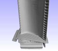 Turbine blade, 1.7 million polys. 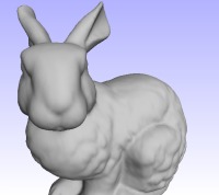 Stanford Bunny, 65k polys. |
| The Clustered Backface Culling technique will be described below. The Implied Multi-Resolution Meshing technique, for specific reasons, will not be discussed in this report. | |
|
Clustered Backface Culling Pseudo code for my implementation of the clustered backface culling algorithm: Pre-processing
   Sort polygons into groups.
   For each group / cluster of polygons
      Compute the Normal Cone for the cluster.
      If the normal cone deviation is too great
         Subdivide group based upon normal orientation
Run-time
   For each group / cluster of polygons
     if the group is completely backfacing (using the normal cone)
        don't render.
     if the group is culled by the view frustum
        don't render.
     Render the group.
The three main areas of technology in the above algorithm is the group sorting, the normal cone computation, and
culling using the normal cone. These will be discussed in further detail in the sections below.
|
|
|
Spatial Grouping For this implementation, I chose to group faces by spatial locality. When loading the model into the display structures, the polygons are sorted using a regular grid of cells. The sample application allows changing the size of this cell grid, but in general one grid size has worked well for most models. The polygons are sorted into one cell only. The images to the right show a display where each cell is colored to illustrate where they begin and end. Any curved boundaries between cells is due to the fact that the spatial division grid is a regular grid and the turbine blade is a curved surface.
Normal Cone Computation To the right is an image which illustrates the cell subdivision handling. The turbine blade has holes drilled along the ends of the blade. The cells which contain these holes would have had normal cones which would not have had much use, so the cell subdivided. The subdivision is illustrated by the fact that the holes have different colored patches inside them, even though the holes are obviously much smaller than the grid cell size. To cull using the normal cone is similar normal backface culling. Instead of simply testing the dot product between the view vector and normal for negative values, we need to consider how large angle is between the normal and the view vector with respect to the maximum deviation in the normal cone. To reject the cluster, the average normal deviated toward the view vector by the maximum deviation must still be backfacing.
View Frustum Culling
|
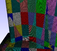 Turbine colored cell view. 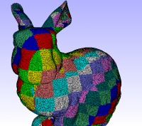 Bunny colored cell view.  Colored cell view showing cells subdivided due to holes.  Wire-frame view of the bunny where cell rejection is more obvious. |
|
Stats So how effective is this? For the turbine blade model, between 21-23% of the model is always rejected by the clustered backface algorithm alone. This is about 400k polygons which we never visit or issue to the graphics pipe. For the Stanford Bunny, around 35% is rejected by the clustered backface algorithm. When you combine the clustered backface culling with the view frustum culling, on the close up images of the turbine 54% of the model has been culled! This amounts to 950K polygons culled! | |
glenn@raudins.com